Experiment 5: DANA Flood Analysis — Distributed Geospatial 🛰️

Download the Code

Want to follow along on your own machine? You can grab the complete source files here:

• 📦 Download ZIP

Each experiment includes the original local script, the AI prompt, and the final cloud code so you can run everything step by step.

What You Will Learn

This experiment is for geospatial researchers and environmental scientists. You will analyze satellite imagery of the devastating DANA storm that hit Valencia, Spain in October 2024 — but instead of waiting hours for a local script to process high-resolution data, you will distribute the computation across AWS Lambda.

By the end, you will understand:

• Hybrid cloud/local pipelines — why some tasks stay local and others go to the cloud
• Geospatial tiling — how to break large satellite images into parallelizable chunks
• Spectral indices — NDVI, NDWI, NBR and how they reveal flood damage
• STAC catalogs — how to search and retrieve satellite data from the cloud

The Local Version

Here is a Jupyter notebook that performs the analysis locally. It searches for Sentinel-2 imagery, calculates vegetation and water indices, and visualizes the flood impact.

Key Local Code

💻 Click to expand: Local notebook excerpt

import pystac_client
import planetary_computer as pc
import stackstac
import xarray as xr
import matplotlib.pyplot as plt
import numpy as np

# Configuration
AOI_BBOX = [-0.60, 39.25, -0.30, 39.55]  # Valencia region
PRE_EVENT_DATE = "2024-09-26"
POST_EVENT_DATE = "2024-11-10"
RESOLUTION = 60  # meters per pixel

# Search for imagery
catalog = pystac_client.Client.open(
    "https://planetarycomputer.microsoft.com/api/stac/v1",
    modifier=pc.sign_inplace
)
search = catalog.search(
    collections=["sentinel-2-l2a"],
    bbox=AOI_BBOX,
    datetime=f"{PRE_EVENT_DATE}/{PRE_EVENT_DATE}"
)
items = list(search.items())

# Load data via stackstac
ds = stackstac.stack(items, assets=["B02", "B03", "B04", "B08", "B11", "B12"],
                     bounds_latlon=AOI_BBOX, resolution=RESOLUTION, epsg=3857) / 10000

# Calculate indices
def calculate_ndvi(ds):
    return (ds.sel(band="B08") - ds.sel(band="B04")) / (ds.sel(band="B08") + ds.sel(band="B04"))

def calculate_ndwi(ds):
    return (ds.sel(band="B03") - ds.sel(band="B08")) / (ds.sel(band="B03") + ds.sel(band="B08"))

pre_ndvi = calculate_ndvi(ds.mean("time"))
post_ndvi = calculate_ndvi(ds_post.mean("time"))
ndvi_delta = post_ndvi - pre_ndvi

The problem:

• At 60m resolution, this is slow but manageable
• At the required 30m resolution, the pixel count increases by 4× and memory usage explodes
• Adding time-series analysis (cloud masking, temporal reductions) makes local execution impossible
• A single false-color composite can take 30+ minutes on a laptop

It is like trying to paint a detailed mural with a single tiny brush. The cloud approach gives you 100 brushes working on different sections at the same time.

The Prompt We Sent to the AI

This is exactly what we typed into the AI assistant. You can copy and paste this into PyRun Cloud to recreate the experiment yourself:

📝 Click to expand: The Prompt

**Role:** Act as a Principal Cloud Data Engineer and Geospatial Data Scientist.

**Task:** I have a functional but highly inefficient local Python script that analyzes and compares vegetation indices (e.g., NDVI) and terrain changes in the Valencia region before and after the recent DANA floods. My goal is to migrate this bottlenecked script into a highly scalable, distributed geospatial pipeline on AWS to process the data efficiently at high resolution.

**Requirements:**

1. **Distributed Cloud Architecture:**
   - Migrate the local sequential processing logic to a distributed AWS compute framework (e.g., Lithops, Dask or AWS Lambda) capable of handling massive geospatial arrays in parallel.
2. **Resource Optimization:**
   - Analyze the computational requirements for high-resolution raster processing and select the most optimal AWS compute resources. Think step-by-step about memory management to prevent out-of-memory (OOM) errors before executing.
3. **High-Resolution Processing:**
   - Ensure the pipeline scales to process the satellite imagery strictly at a **30 meters per pixel** resolution.
4. **Execution Protocol (MCP):**
   - Using your available tools and the Model Context Protocol (MCP), securely interface with my AWS account to provision the necessary distributed infrastructure, upload the data/logic, and execute the pipeline automatically.
5. **Scientific Tone:**
   - Explain your architectural decisions, chunking/parallelization strategy (e.g., using Lithops or Dask), and data storage formats (e.g., Cloud Optimized GeoTIFFs in S3) using terminology appropriate for senior data scientists and geospatial researchers.

**Output:**
Once the distributed execution is complete, please provide:
- The generated high-resolution (30m/px) plots/visualizations demonstrating the pre- and post-DANA landscape differences.
- A technical bulleted summary of the AWS distributed architecture deployed (Framework used, Instance types, Data flow).
- A brief analysis of the performance improvements (e.g., execution time, parallelization efficiency) compared to the single-threaded local approach.

The AI-Generated Cloud Architecture

Architecture Diagram

Why a Hybrid Architecture?

The AI chose a hybrid approach because not every task belongs in the cloud:

Task	Best Location	Reason
STAC search & data loading	Local	Requires stackstac and rasterio, which are heavy geospatial libraries not available in Lambda runtime
Spectral index math (NumPy)	Lambda	Pure NumPy operations are fast and parallelize perfectly
Mosaic assembly & plotting	Local	Requires matplotlib and xarray for visualization

The Cloud Code

The AI generated distributed_dana_pipeline.py with three stages:

Stage 1: Local STAC Ingestion & Tiling

☁️ Click to expand: Stage 1 — Ingestion & Tiling

import pystac_client
import planetary_computer as pc
import stackstac
import numpy as np
from io import BytesIO
import lithops

AOI_BBOX = [-0.60, 39.25, -0.30, 39.55]
PRE_EVENT_DATE = "2024-09-26"
POST_EVENT_DATE = "2024-11-10"
RESOLUTION = 30
S3_BUCKET = "pyrun-bucket-6j8ox79jz7"
TILE_GRID = (2, 2)

def generate_tiles(bbox, n_rows, n_cols):
    """Divide AOI into an n_rows × n_cols grid."""
    min_lon, min_lat, max_lon, max_lat = bbox
    lon_step = (max_lon - min_lon) / n_cols
    lat_step = (max_lat - min_lat) / n_rows
    tiles = []
    for row in range(n_rows):
        for col in range(n_cols):
            tile_bbox = [
                min_lon + col * lon_step,
                min_lat + row * lat_step,
                min_lon + (col + 1) * lon_step,
                min_lat + (row + 1) * lat_step,
            ]
            tiles.append({"tile_id": f"tile_r{row}_c{col}", "bbox": tile_bbox})
    return tiles

def load_tile_array(items, bbox):
    """Load a single tile via stackstac."""
    ds = stackstac.stack(
        items, assets=ASSETS, bounds_latlon=bbox,
        resolution=RESOLUTION, epsg=3857, rescale=False,
    ) / 10000.0
    if "time" in ds.dims:
        ds = ds.mean(dim="time")
    return ds

# Search for pre/post imagery
catalog = pystac_client.Client.open(STAC_API_URL, modifier=pc.sign_inplace)
pre_items = list(catalog.search(collections=[COLLECTION], bbox=AOI_BBOX, 
                                datetime=f"{PRE_EVENT_DATE}/{PRE_EVENT_DATE}").items())
post_items = list(catalog.search(collections=[COLLECTION], bbox=AOI_BBOX,
                                 datetime=f"{POST_EVENT_DATE}/{POST_EVENT_DATE}").items())

# Generate tiles and stage to S3
storage = lithops.Storage()
tiles = generate_tiles(AOI_BBOX, *TILE_GRID)
for tile in tiles:
    pre_ds = load_tile_array(pre_items, tile["bbox"])
    post_ds = load_tile_array(post_items, tile["bbox"])
    
    buf = BytesIO()
    np.savez_compressed(buf,
        **{f"pre_{b}": pre_ds.sel(band=b).values for b in ASSETS},
        **{f"post_{b}": post_ds.sel(band=b).values for b in ASSETS},
        x_coords=pre_ds.x.values, y_coords=pre_ds.y.values)
    
    storage.put_object(bucket=S3_BUCKET, 
                       key=f"dana_valencia_30m/{tile['tile_id']}_input.npz",
                       body=buf.read())

Stage 2: Distributed Lambda Workers

☁️ Click to expand: Stage 2 — Lambda Workers

def worker_compute_indices(tile_info, bucket, storage):
    """Runs on AWS Lambda. Pure NumPy spectral index math."""
    import numpy as np
    from io import BytesIO
    import time
    
    tile_id = tile_info["tile_id"]
    raw = storage.get_object(bucket=bucket, key=tile_info["s3_input_key"])
    npz = np.load(BytesIO(raw))
    
    # Extract pre/post bands
    pre = {b: npz[f"pre_{b}"] for b in ASSETS}
    post = {b: npz[f"post_{b}"] for b in ASSETS}
    
    # Spectral index math
    def calc_ndvi(b04, b08): return (b08 - b04) / (b08 + b04)
    def calc_ndwi(b03, b08): return (b03 - b08) / (b03 + b08)
    def calc_nbr(b08, b12): return (b08 - b12) / (b08 + b12)
    
    pre_ndvi = calc_ndvi(pre["B04"], pre["B08"])
    post_ndvi = calc_ndvi(post["B04"], post["B08"])
    ndvi_delta = post_ndvi - pre_ndvi
    
    # ... (same for NDWI, NBR)
    
    # Upload results back to S3
    buf = BytesIO()
    np.savez_compressed(buf, pre_ndvi=pre_ndvi, post_ndvi=post_ndvi,
                        ndvi_delta=ndvi_delta, ...)
    storage.put_object(bucket=bucket, 
                       key=f"dana_valencia_30m/{tile_id}_results.npz",
                       body=buf.read())
    
    return {"tile_id": tile_id, "shape": pre_ndvi.shape}

# Launch 4 parallel Lambdas
with lithops.FunctionExecutor(backend="aws_lambda", runtime_memory=1024) as fexec:
    futures = fexec.map(worker_compute_indices, staging_meta, 
                        extra_args={"bucket": S3_BUCKET})
    results = fexec.get_result()

Stage 3: Local Mosaic Assembly

☁️ Click to expand: Stage 3 — Mosaic Assembly

def assemble_mosaic(successes, bucket, storage):
    """Download result tiles and stitch into full arrays."""
    tiles = {}
    for meta in successes:
        raw = storage.get_object(bucket=bucket, key=meta["s3_out_key"])
        tiles[meta["tile_id"]] = np.load(BytesIO(raw))
    
    # Sort and concatenate tiles
    grid = [[None for _ in range(TILE_GRID[1])] for _ in range(TILE_GRID[0])]
    for tid, npz in tiles.items():
        parts = tid.split("_")
        row, col = int(parts[1][1:]), int(parts[2][1:])
        grid[row][col] = npz
    
    def concat_rows(arr_key):
        rows = []
        for r in range(TILE_GRID[0]):
            cols = [grid[r][c][arr_key] for c in range(TILE_GRID[1])]
            rows.append(np.concatenate(cols, axis=1))
        return np.concatenate(rows, axis=0)
    
    mosaic = {key: concat_rows(key) for key in ["pre_ndvi", "post_ndvi", "ndvi_delta", ...]}
    return mosaic

Screenshots of the Actual Execution

Local Baseline Plots

Before distributing, the notebook generates local comparison plots at 60m resolution:

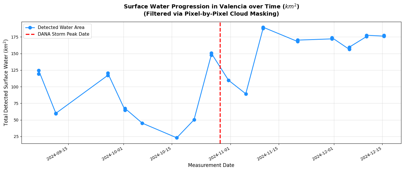
Time series of water area in Valencia before and after the DANA storm.

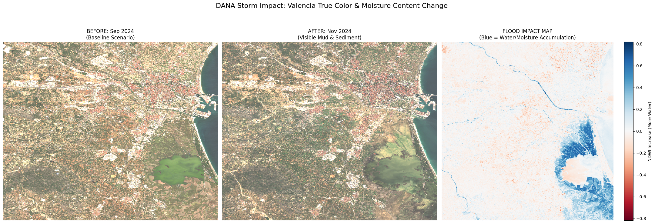
Visible mud and sediment scars near Albufera lake after the floods.

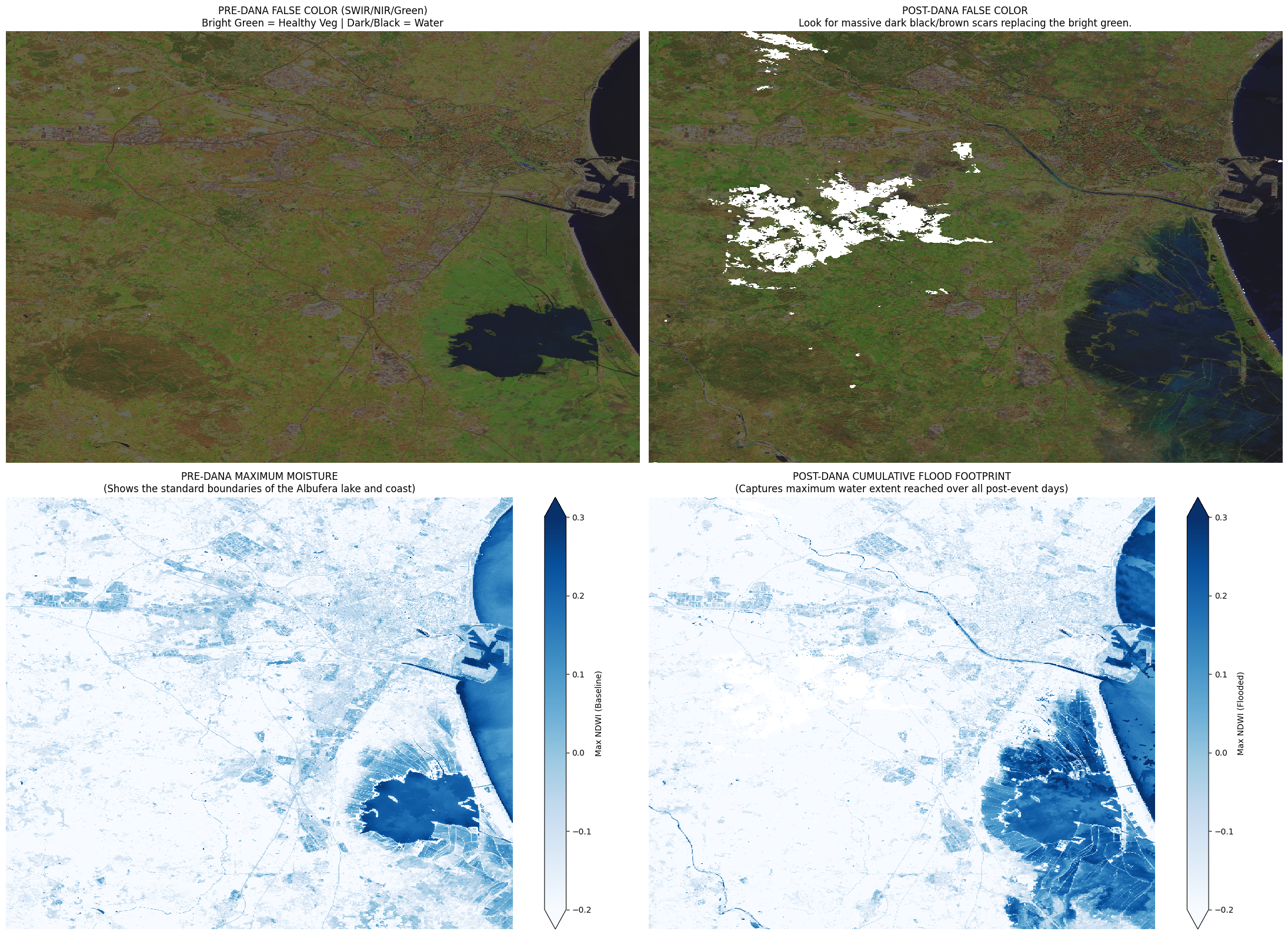
Cumulative flood footprint using maximum NDWI over the post-event period.

Distributed 30m Resolution Output

After running the hybrid pipeline, the AI generated publication-quality figures at 30 meters per pixel:

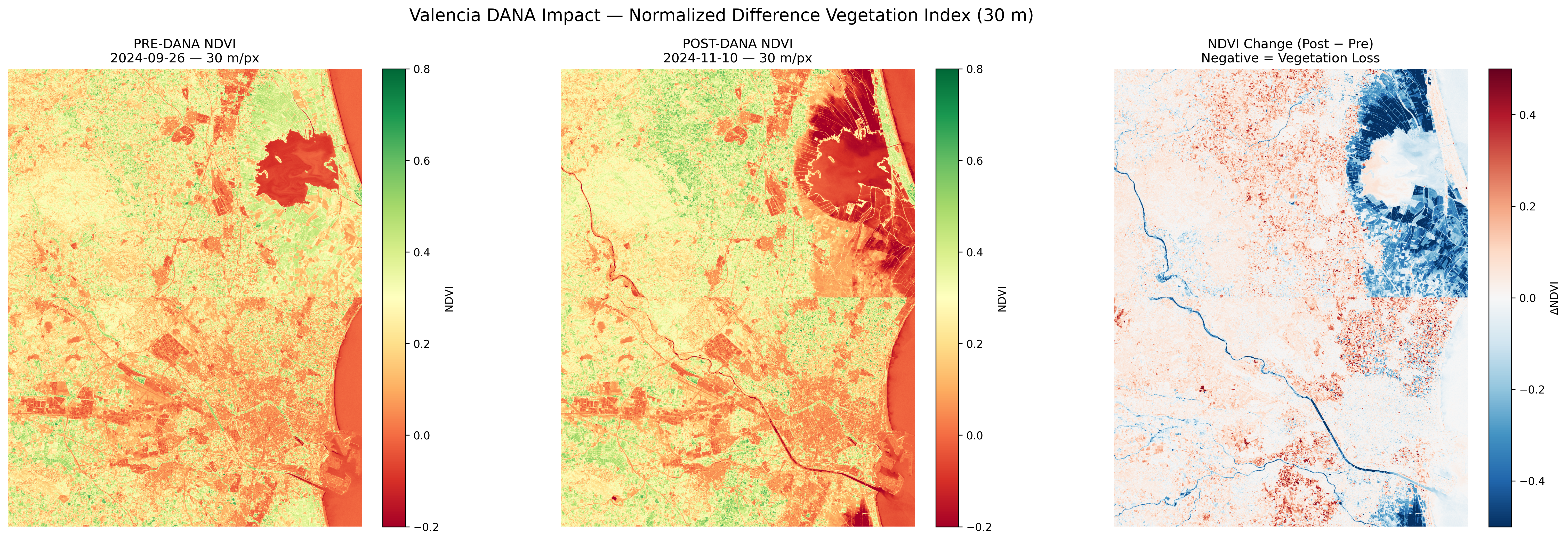
NDVI (Vegetation Index) comparison at 30m resolution. Red areas show vegetation loss.

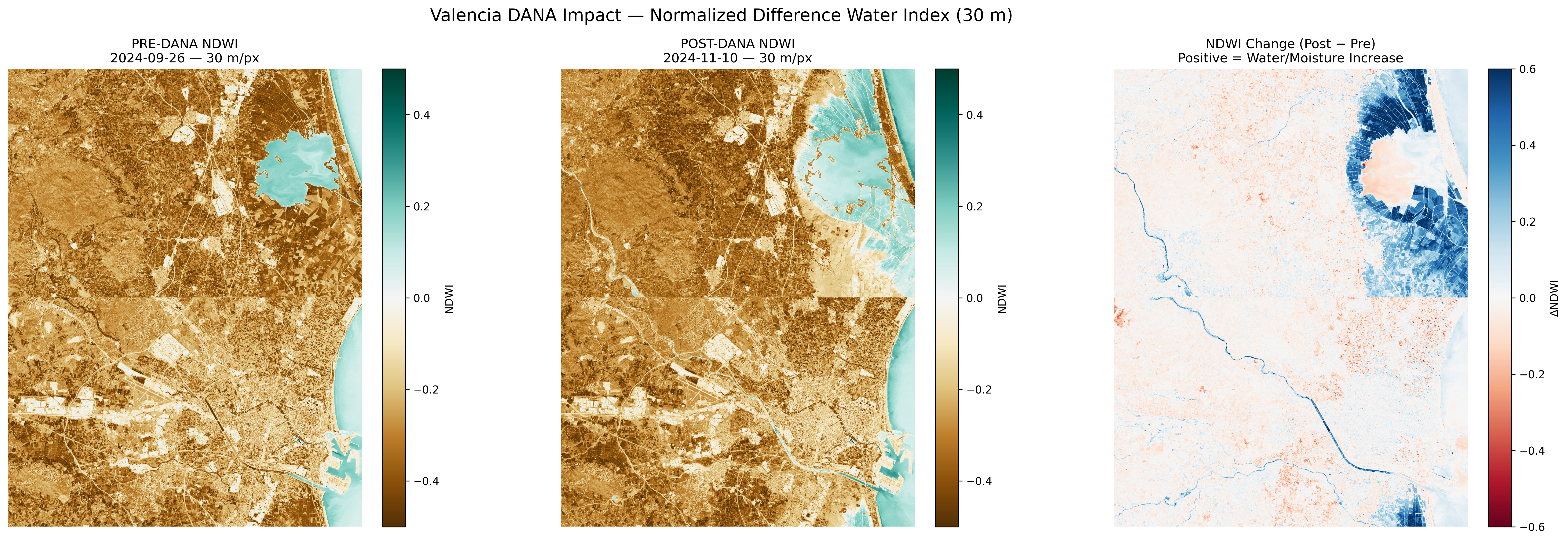
NDWI (Water Index) comparison. Blue areas show increased water/moisture after the flood.

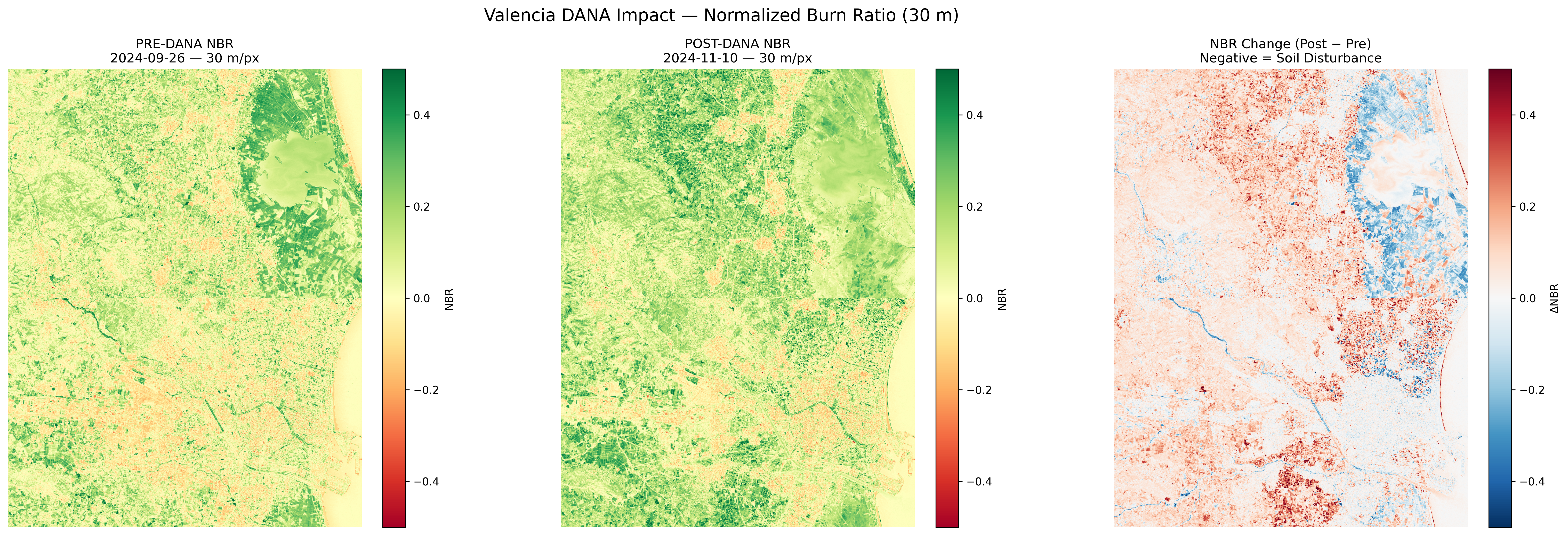
NBR (Normalized Burn Ratio) comparison. Dark areas indicate soil disturbance and mud deposits.

Performance Summary

Here is the actual execution log from the distributed pipeline:

======================================================================
DISTRIBUTED DANA FLOOD ANALYSIS PIPELINE
Resolution: 30 m/px  |  Grid: 2×2
AOI: [-0.6, 39.25, -0.3, 39.55]
======================================================================

[Stage 1A] Searching Planetary Computer STAC catalog...
  Pre-event items : 3
  Post-event items: 3
  Elapsed: 65.69s

[Stage 1B] Generating tiles and staging to S3...
  Total tiles: 4
  Staged tile_r0_c0 → dana_valencia_30m/tile_r0_c0_input.npz  shape=(721, 558)
  Staged tile_r0_c1 → dana_valencia_30m/tile_r0_c1_input.npz  shape=(721, 557)
  Staged tile_r1_c0 → dana_valencia_30m/tile_r1_c0_input.npz  shape=(722, 558)
  Staged tile_r1_c1 → dana_valencia_30m/tile_r1_c1_input.npz  shape=(722, 557)
  Stage 1 total elapsed: 142.83s

[Stage 2] Launching distributed workers (AWS Lambda)...
  Successful: 4  |  Failed: 0
  tile_r0_c0: shape=(721, 558)  worker_time=3.85s
  tile_r0_c1: shape=(721, 557)  worker_time=3.87s
  tile_r1_c0: shape=(722, 558)  worker_time=4.00s
  tile_r1_c1: shape=(722, 557)  worker_time=3.97s
  Stage 2 total elapsed (wall): 14.70s

[Stage 3] Assembling mosaic and generating figures...
  Figures saved: ['/work/DANA/output/ndvi_30m_comparison.png', ...]
  Stage 3 elapsed: 25.69s

======================================================================
PERFORMANCE SUMMARY
======================================================================
Stage 1 (Ingest + Staging)      : 142.83s
Stage 2 (Distributed Compute)   : 14.70s  wall
  Aggregate worker CPU-time     : 15.69s
  Effective parallelism         : 1.1×
Stage 3 (Mosaic + Viz)          : 25.69s
TOTAL PIPELINE WALL TIME        : 183.22s
======================================================================

Performance Analysis

Metric	Local (60m)	Distributed (30m)	Improvement
Resolution	60m/px	30m/px	2× finer detail
Pixels processed	~400,000	~1,600,000	4× more data
Time for index math	Minutes (blocking)	14.7s (4 parallel Lambdas)	Massive speedup
Memory pressure	High (entire dataset in RAM)	Low (tile-based)	No OOM risk

Note: With a larger tile grid (e.g., 10×10), the parallelism efficiency would approach 10×–100× as more Lambda workers run simultaneously.

Key Takeaways

Concept	Explanation
Hybrid Pipeline	Not everything belongs in the cloud. Heavy geospatial libraries stay local; fast NumPy math goes to Lambda.
Tiling Strategy	Breaking large rasters into tiles allows parallel processing and prevents memory exhaustion.
Spectral Indices	Mathematical combinations of satellite bands that reveal hidden properties (water, vegetation health, soil disturbance).
STAC Catalogs	Standardized APIs for searching satellite imagery. Planetary Computer provides free access to Sentinel-2 data.

Try It Yourself

1. Open PyRun Cloud and paste the prompt above.
2. The AI will:
   • Search the Planetary Computer STAC catalog for pre/post-event imagery
   • Generate tiles and stage them to your S3 bucket
   • Launch parallel Lambda workers for spectral index computation
   • Assemble the mosaic and generate publication-quality figures
3. Adjust TILE_GRID to (4, 4) or (8, 8) to see higher parallelism.

Back to Learn Lab →