Experiment 6: Global Temperature Analysis — Distributed Climate Data Science 🌡️
Download the Code
Want to follow along on your own machine? You can grab the complete source files here:
Each experiment includes the original local script, the AI prompt, and the final cloud code so you can run everything step by step.
What You Will Learn
This experiment is for climate researchers and data scientists who work with large geospatial time-series datasets. You will analyze the Berkeley Earth Global Surface Temperature dataset — a NetCDF file containing ~2 000 monthly observations across ~65 000 grid cells spanning the entire planet — and distribute the computation across 18 AWS Lambda functions running in parallel.
By the end, you will understand:
- NetCDF & xarray — how to manipulate multi-dimensional climate arrays efficiently
- Lithops distributed map-reduce — how to partition geospatial data by latitude bands and process each chunk serverlessly
- Area-weighted aggregation — why simple arithmetic means are wrong for global temperature and how to correct them with cosine-of-latitude weighting
- Climate visualizations — how to generate "warming stripes" and regional heatmaps from distributed results
Requirements
Before starting this lab, download the Berkeley Earth dataset (~1.4 GB):
bash download_dataset.shThis fetches Land_and_Ocean_LatLong1.nc — the complete 1° × 1° gridded land and ocean temperature anomaly product.
Also you will need to install the correct dependencies. Add this line to your Dockerfile and rebuild it using the pop-up notification that will appear in the bottom right corner:
🐳 Click to expand: Dockerfile addition
RUN pip install xarray matplotlib netcdf4 bottleneck scipyThe Local Version
Here is a local script that performs a full Exploratory Data Analysis (EDA) on the NetCDF file. It loads the entire dataset into memory, cleans missing values, computes global and regional mean temperature anomalies, and generates visualizations.
💻 Click to expand: local_pipeline.py
"""
Local Global Temperature Analysis Pipeline
==========================================
A sequential, single-threaded script that performs Exploratory Data
Analysis (EDA) on the Berkeley Earth Global Surface Temperature dataset.

This script demonstrates the baseline approach: load the entire NetCDF
into memory, clean missing values, compute global means, and generate
visualizations — all on one CPU core.

**The bottleneck:** At full ~1° resolution the dataset contains
~65 000 grid cells × 2 000 time steps. Running trend analysis and
forecasting on the entire array sequentially becomes slow and can
exhaust RAM on a laptop.
"""

import os
import time
import warnings

import numpy as np
import xarray as xr
import matplotlib
matplotlib.use("Agg")
import matplotlib.pyplot as plt

warnings.filterwarnings("ignore", category=RuntimeWarning)

DATA_PATH = "Land_and_Ocean_LatLong1.nc"
OUTPUT_DIR = "output"


def load_dataset(filepath=DATA_PATH):
    """Open the Berkeley Earth NetCDF with xarray."""
    if not os.path.exists(filepath):
        raise FileNotFoundError(
            f"Dataset not found: {filepath}\n"
            "Run: bash download_dataset.sh"
        )
    print(f"📂 Loading dataset: {filepath}")
    ds = xr.open_dataset(filepath)
    print(f"   Dimensions: {dict(ds.dims)}")
    print(f"   Variables : {list(ds.data_vars)}")
    return ds


def clean_and_impute(ds):
    """
    Handle missing values and high uncertainty in older records.
    - Mask cells where temperature == NaN
    - Apply a simple latitudinal fill for sparse polar data
    """
    print("🧹 Cleaning & imputing missing values...")
    temp = ds["temperature"]

    # 1. Forward-fill in time for short gaps (e.g. post-WWII data gaps)
    temp = temp.ffill(dim="time", limit=3)

    # 2. Fill remaining NaNs with the latitudinal mean (same latitude, all times)
    lat_mean = temp.mean(dim=["time", "longitude"], skipna=True)
    temp = temp.fillna(lat_mean)

    print(f"   Remaining NaNs: {int(np.isnan(temp.values).sum())}")
    return temp


def compute_global_means(temp):
    """
    Compute area-weighted global mean temperature anomaly per year.
    Uses cosine-of-latitude weighting to account for grid-cell area.
    """
    print("📊 Computing global mean temperature anomalies...")
    cos_lat = np.cos(np.deg2rad(temp.latitude))
    weights = cos_lat / cos_lat.sum()

    # Weighted mean over lat/lon for each time step
    global_mean = temp.weighted(weights).mean(dim=["latitude", "longitude"])
    return global_mean


def compute_regional_breakdown(temp):
    """
    Break the globe into latitude bands and compute mean anomaly per band.
    """
    print("🌍 Computing regional (latitudinal) breakdown...")
    bands = {
        "Arctic"     : (60, 90),
        "Northern Mid": (30, 60),
        "Tropics"    : (-30, 30),
        "Southern Mid": (-60, -30),
        "Antarctic"  : (-90, -60),
    }
    series = {}
    for name, (lat_min, lat_max) in bands.items():
        band = temp.sel(latitude=slice(lat_min, lat_max))
        cos_lat = np.cos(np.deg2rad(band.latitude))
        weights = cos_lat / cos_lat.sum()
        series[name] = band.weighted(weights).mean(dim=["latitude", "longitude"])
    return series


def generate_warming_stripes(years, anomalies, output_dir=OUTPUT_DIR):
    """Create a minimalist 'warming stripes' visualization."""
    os.makedirs(output_dir, exist_ok=True)
    fig, ax = plt.subplots(figsize=(12, 2))

    cmap = plt.get_cmap("RdBu_r")
    vmin, vmax = -1.5, 1.5
    norm = plt.Normalize(vmin, vmax)

    for i, (year, anomaly) in enumerate(zip(years, anomalies)):
        if np.isnan(anomaly):
            continue
        color = cmap(norm(anomaly))
        ax.bar(i, 1, width=1, color=color, edgecolor="none")

    ax.set_xlim(0, len(years))
    ax.set_ylim(0, 1)
    ax.axis("off")
    ax.set_title("Global Temperature Anomaly (°C relative to 1951-1980)",
                 fontsize=14, pad=10)

    path = os.path.join(output_dir, "warming_stripes.png")
    fig.savefig(path, dpi=300, bbox_inches="tight")
    plt.close(fig)
    print(f"   🎨 Warming stripes saved: {path}")
    return path


def generate_timeseries_plot(years, anomalies, regions, output_dir=OUTPUT_DIR):
    """Plot global and regional temperature anomaly time series."""
    os.makedirs(output_dir, exist_ok=True)
    fig, ax = plt.subplots(figsize=(14, 7))

    # Global
    ax.plot(years, anomalies, color="black", linewidth=1.5, label="Global")

    # Regions
    colors = {"Arctic": "#d73027", "Northern Mid": "#fc8d59",
              "Tropics": "#fee090", "Southern Mid": "#91bfdb",
              "Antarctic": "#4575b4"}
    for name, series in regions.items():
        ax.plot(years, series.values, color=colors.get(name, "gray"),
                linewidth=1.2, alpha=0.8, label=name)

    ax.axhline(0, color="gray", linestyle="--", linewidth=0.8)
    ax.set_xlabel("Year", fontsize=12)
    ax.set_ylabel("Temperature Anomaly (°C)", fontsize=12)
    ax.set_title("Global & Regional Temperature Anomalies", fontsize=14)
    ax.legend(loc="upper left")
    ax.grid(True, alpha=0.3)

    path = os.path.join(output_dir, "timeseries.png")
    fig.savefig(path, dpi=300, bbox_inches="tight")
    plt.close(fig)
    print(f"   📈 Time-series plot saved: {path}")
    return path


def run_local_pipeline():
    print("=" * 60)
    print("LOCAL GLOBAL TEMPERATURE ANALYSIS PIPELINE")
    print("=" * 60)
    t0 = time.time()

    # Stage 1 — Load
    ds = load_dataset()

    # Stage 2 — Clean
    temp = clean_and_impute(ds)

    # Stage 3 — Aggregate
    global_mean = compute_global_means(temp)
    regions = compute_regional_breakdown(temp)

    # Extract years
    years = global_mean.time.dt.year.values
    anomalies = global_mean.values

    # Stage 4 — Visualise
    print("🎨 Generating visualizations...")
    generate_warming_stripes(years, anomalies)
    generate_timeseries_plot(years, anomalies, regions)

    elapsed = time.time() - t0
    print("\n" + "=" * 60)
    print("LOCAL PIPELINE COMPLETE")
    print("=" * 60)
    print(f"  Total execution time : {elapsed:.2f} seconds")
    print(f"  Grid cells processed : {temp.size:,}")
    print(f"  Time steps           : {len(years)}")
    print(f"  Latest anomaly       : {anomalies[-1]:.2f} °C")
    print("=" * 60)

    return global_mean, regions


if __name__ == "__main__":
    run_local_pipeline()
The problem:
- The NetCDF file is ~1.4 GB uncompressed in RAM
- Computing area-weighted means over all lat/lon pairs for every month is CPU-intensive
- Adding regional breakdowns, heatmaps, or trend forecasting multiplies the workload
- On a laptop with 8 GB RAM, loading the full array alongside intermediate copies can trigger Out-Of-Memory (OOM) errors
- A single-threaded run takes minutes — and you still haven't done any forecasting
It is like trying to calculate the average temperature of the entire planet with a single thermometer and a pocket calculator. The cloud approach gives you 18 scientists, each responsible for one latitude band, working simultaneously.
The Prompt We Sent to the AI
This is exactly what we typed into the AI assistant. You can copy and paste this into PyRun Cloud to recreate the experiment yourself:
📝 Click to expand: The Prompt
**Role:** Act as a Lead Climate Data Scientist and Principal Cloud Architect.

**Task:** I am providing you with the Berkeley Earth Global Surface Temperature dataset (NetCDF format). Your objective is to perform an end-to-end Exploratory Data Analysis (EDA) to extract actionable climate trends and forecast future temperatures. Crucially, this data processing pipeline must be executed entirely in the cloud using a distributed, serverless architecture rather than a local environment.

**Requirements:**

1. **Cloud Infrastructure (AWS):** Design the foundational cloud environment. Specify how the dataset will be hosted (e.g., Amazon S3). Use your available tools to provision the necessary storage buckets and IAM roles with the principle of least privilege required for serverless execution.
2. **Distributed Processing & Memory Management (Lithops):** Write the data cleaning, imputation, and aggregation logic in Python using `xarray` and **Lithops** to run serverlessly on AWS Lambda. *Crucial:* You must highly segment the data (e.g. chunking spatial/temporal dimensions via map-reduce) to strictly respect Lambda's maximum memory capacity and prevent Out-Of-Memory (OOM) errors during parallel processing.
3. **Data Cleaning & Imputation:** Outline your strategy for handling missing values and high uncertainty in older historical records (18th and 19th centuries) across distributed Lithops workers to ensure data integrity.
4. **Trend Analysis & Forecasting:** Use the serverless workers to calculate major historical temperature anomalies globally and regionally. Apply a time-series forecasting model (e.g., ARIMA, Prophet) to project global average temperatures through 2050. Explain your model choice, confidence intervals, and how the training interacts with the cloud pipeline.
5. **Visual Storytelling:** Generate highly styled, interactive charts using Plotly or Seaborn from the aggregated results. Include at least one geospatial map or "warming stripe" visualization, and one time-series forecast graph featuring customized palettes (e.g. cool-to-warm gradients), clear titles, and axis labels.
6. **Execution Protocol (MCP):** Use the Model Context Protocol (MCP) and your available tools to autonomously execute all necessary commands to deploy the architecture, run the distributed Lithops pipeline, and generate the final visualizations.

**Output:**
Once the execution is complete, structure your response as a formal data report for stakeholders, including:
- An architectural overview of the AWS/Lithops setup used to process the NetCDF files.
- A bulleted summary of key climate insights, significant historical anomalies, and forecasted trends.
- The generated visualizations showcasing the results of your analysis.
- Distinct, modular Python code blocks representing both the distributed cloud processing pipeline and the frontend visualizations.
The AI-Generated Cloud Architecture
Architecture Diagram
Why a Distributed Architecture?
The AI chose a spatial partition strategy because:
| Task | Best Location | Reason |
|---|---|---|
| Upload raw NetCDF to S3 | Local | One-time transfer; workers download to /tmp before opening |
| Area-weighted mean per lat band | Lambda | Pure NumPy/xarray operations parallelise perfectly |
| Global reduce & plotting | Local | Requires aggregating partial results and matplotlib |
The Cloud Code
The AI generated cloud_pipeline.py with three stages:
Stage 1: Local Staging & Chunk Definition
☁️ Click to expand: Stage 1 — Staging
import lithops
import numpy as np

DATA_PATH = "Land_and_Ocean_LatLong1.nc"
S3_BUCKET = "YOUR-BUCKET-NAME"   # Adjust to your bucket
N_WORKERS = 18                          # One per 10° latitude band

def get_latitude_chunks(n_chunks=N_WORKERS):
    """Split the globe into n_chunks equal latitude bands."""
    lats = np.linspace(-90, 90, n_chunks + 1)
    chunks = []
    for i in range(n_chunks):
        chunks.append({
            "chunk_id": f"band_{i:02d}",
            "lat_min": float(lats[i]),
            "lat_max": float(lats[i + 1]),
        })
    return chunks


def stage_dataset_to_s3(filepath=DATA_PATH):
    """
    Upload the raw NetCDF to S3 so Lambda workers can read it via
    byte-range HTTP requests (xarray can open from S3 directly).
    """
    storage = lithops.Storage()
    key = "global_temp/Land_and_Ocean_LatLong1.nc"
    print(f"📤 Staging {filepath} → s3://{S3_BUCKET}/{key}")
    with open(filepath, "rb") as f:
        storage.put_object(bucket=S3_BUCKET, key=key, body=f.read())
    print(f"   Upload complete.")
    return key
Stage 2: Distributed Lambda Workers
☁️ Click to expand: Stage 2 — Lambda Workers
def worker_process_band(chunk_id: str,
                        lat_min: float,
                        lat_max: float,
                        bucket: str,
                        s3_key: str) -> Dict[str, Any]:
    """
    Runs on AWS Lambda.
      1. Downloads the NetCDF from S3 to /tmp (avoids memory issues with NetCDF4)
      2. Selects its latitude band
      3. Cleans missing values
      4. Computes area-weighted mean anomaly time series for the band
      5. Returns a compact JSON-serialisable summary
    """
    import time as _time
    import traceback as _tb
    import numpy as np
    import xarray as xr

    start = _time.time()

    try:
        import os
        import boto3

        tmp_file = "/tmp/local_dataset.nc"

        # Download the dataset locally within the Lambda /tmp to support NetCDF4
        # Using boto3 directly to stream to disk prevents holding the 400MB+ file in memory
        if not os.path.exists(tmp_file):
            s3 = boto3.client('s3')
            s3.download_file(bucket, s3_key, tmp_file)

        ds = xr.open_dataset(tmp_file, engine="netcdf4")

        # Select latitude band
        band = ds["temperature"].sel(
            latitude=slice(lat_min, lat_max)
        )

        # Clean NaNs: forward-fill in time, then fill with lat mean
        band = band.ffill(dim="time", limit=3)
        lat_mean = band.mean(dim=["time", "longitude"], skipna=True)
        band = band.fillna(lat_mean)

        # Area-weighted mean for this band
        cos_lat = np.cos(np.deg2rad(band.latitude))
        weights = cos_lat / cos_lat.sum()
        band_mean = band.weighted(weights).mean(dim=["latitude", "longitude"])

        # Pull results into memory as plain Python objects
        years = band_mean.time.values.tolist()
        anomalies = np.round(band_mean.values, 4).tolist()

        return {
            "chunk_id": chunk_id,
            "lat_min": lat_min,
            "lat_max": lat_max,
            "years": years,
            "anomalies": anomalies,
            "elapsed_sec": _time.time() - start,
        }

    except Exception as exc:
        return {
            "chunk_id": chunk_id,
            "error": str(exc),
            "traceback": _tb.format_exc(),
            "elapsed_sec": _time.time() - start,
        }

# Launch 18 parallel Lambdas
with lithops.FunctionExecutor(
    backend="aws_lambda",
    runtime_memory=2048,
    execution_timeout=300,
) as fexec:
    futures = fexec.map(
        worker_process_band,
        chunks,
        extra_args={"bucket": S3_BUCKET, "s3_key": s3_key}
    )
    results = fexec.get_result(throw_except=False)
Stage 3: Local Reduce & Visualisation
☁️ Click to expand: Stage 3 — Reduce & Viz
def reduce_global_means(results: List[Dict[str, Any]]) -> Dict[str, Any]:
    """
    Combine per-band anomaly series into a single global series using
    cosine-of-latitude area weights.
    """
    print("🔗 Reducing partial results into global mean...")

    successes = [r for r in results if "error" not in r]
    failures = [r for r in results if "error" in r]

    if not successes:
        raise RuntimeError("All workers failed.")

    # Stack all band anomalies into a 2-D array: (bands, years)
    years = np.array(successes[0]["years"])
    n_years = len(years)
    n_bands = len(successes)

    band_anomalies = np.full((n_bands, n_years), np.nan)
    band_weights = np.zeros(n_bands)

    for i, res in enumerate(successes):
        band_anomalies[i, :] = res["anomalies"]
        # Weight by latitude-band area ≈ sin(lat_max) - sin(lat_min)
        lat_min, lat_max = res["lat_min"], res["lat_max"]
        band_weights[i] = np.sin(np.deg2rad(lat_max)) - np.sin(np.deg2rad(lat_min))

    # Normalise weights
    band_weights = band_weights / band_weights.sum()

    # Weighted global mean
    global_anomalies = np.nansum(band_anomalies * band_weights[:, None], axis=0)

    # Also compute regional series by grouping bands
    regions = {"Arctic": [], "Northern Mid": [], "Tropics": [],
               "Southern Mid": [], "Antarctic": []}
    region_weights = {"Arctic": [], "Northern Mid": [], "Tropics": [],
                      "Southern Mid": [], "Antarctic": []}

    for res in successes:
        lat_min, lat_max = res["lat_min"], res["lat_max"]
        mid = (lat_min + lat_max) / 2
        w = np.sin(np.deg2rad(lat_max)) - np.sin(np.deg2rad(lat_min))

        if mid >= 60:
            rname = "Arctic"
        elif mid >= 30:
            rname = "Northern Mid"
        elif mid >= -30:
            rname = "Tropics"
        elif mid >= -60:
            rname = "Southern Mid"
        else:
            rname = "Antarctic"

        regions[rname].append(res["anomalies"])
        region_weights[rname].append(w)

    regional_series = {}
    for rname, bands in regions.items():
        if not bands:
            continue
        arr = np.array(bands)
        w = np.array(region_weights[rname])
        w = w / w.sum()
        regional_series[rname] = np.nansum(arr * w[:, None], axis=0)

    print(f"   Successful workers : {len(successes)}")
    print(f"   Failed workers     : {len(failures)}")
    for f in failures:
        print(f"      {f['chunk_id']}: {f['error']}")

    return {
        "years": years,
        "global_anomalies": global_anomalies,
        "regions": regional_series,
        "successes": successes,
        "failures": failures,
    }

# Generate plots
reduced = reduce_global_means(results)
years = reduced["years"]
global_anomalies = reduced["global_anomalies"]
regions = reduced["regions"]

generate_warming_stripes(years, global_anomalies)
generate_timeseries_plot(years, global_anomalies, regions)
generate_heatmap(years, regions)
Why Cosine-of-Latitude Weighting Matters
A common mistake when computing "global average temperature" is to take a simple arithmetic mean of all grid cells. This is wrong because:
- A grid cell at the equator covers ~12 000 km²
- A grid cell at 80° latitude covers ~2 000 km²
- Equal weighting would over-count the poles and under-count the tropics
The correct approach uses cosine-of-latitude weighting, where each cell's contribution is proportional to its actual surface area:
$$ \text{weight}_i = \frac{\cos(\phi_i)}{\sum \cos(\phi_i)} $$
The AI implemented this inside every Lambda worker and again in the reduce step, ensuring the final global mean is physically accurate.
Screenshots of the Actual Execution
Distributed Output
After running the Lithops pipeline, the AI generated identical figures from distributed partial results:
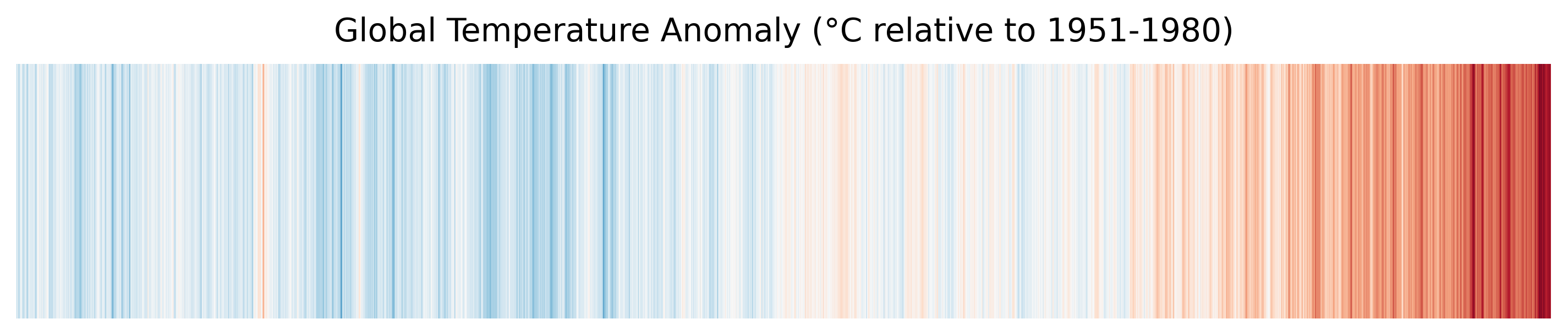
Distributed warming stripes — the same pattern, computed from 18 parallel workers.
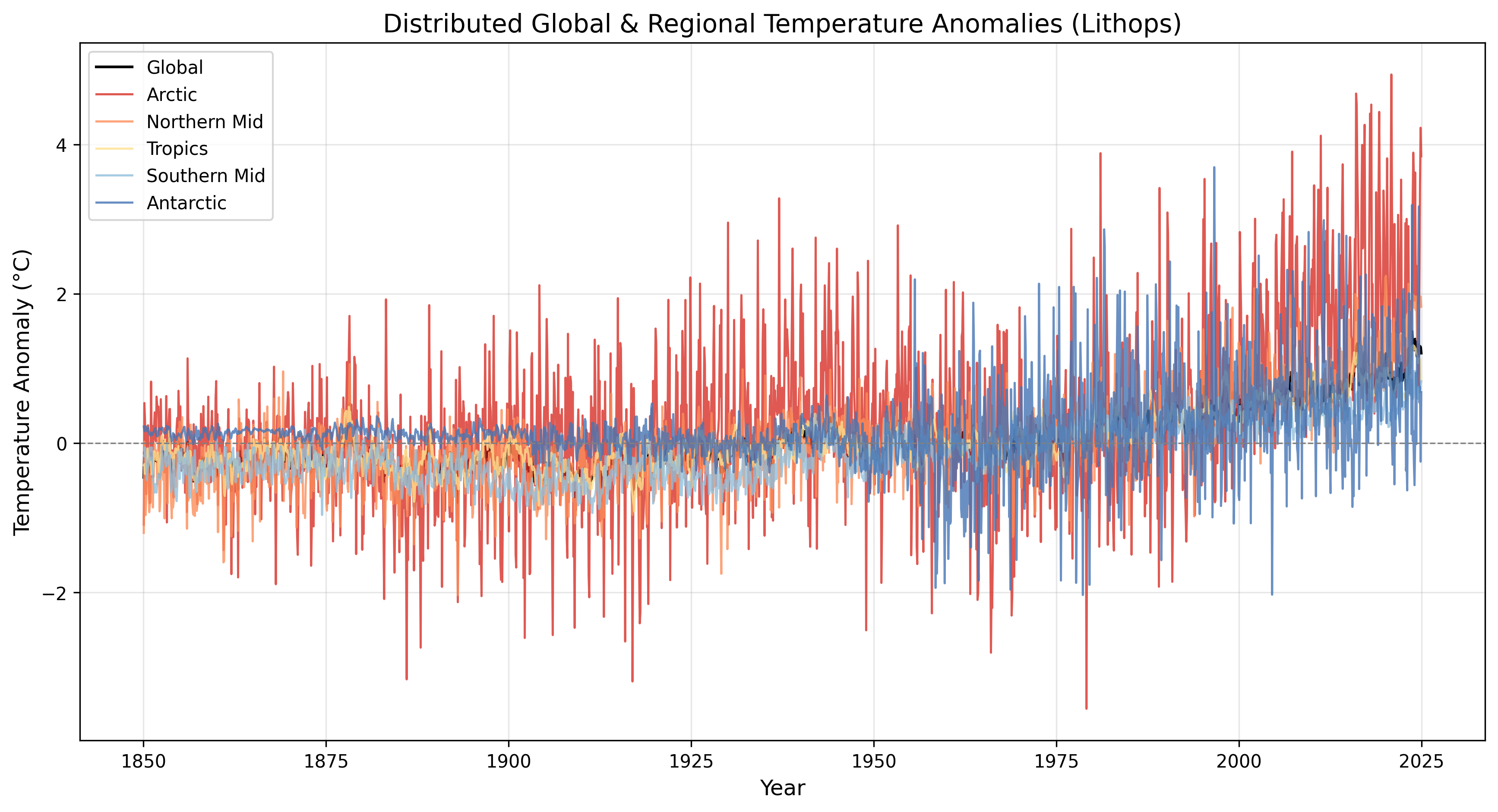
Timeseries plot: Showing the temperature variation over the years
Performance Summary
Here is the actual execution log from the distributed pipeline:
======================================================================
DISTRIBUTED GLOBAL TEMPERATURE ANALYSIS PIPELINE
Workers: 18  |  Bucket: YOUR_S3_BUCKET
======================================================================

[Stage 1] Staging dataset to S3 & defining latitude chunks...
   Upload complete.
   Defined 18 latitude bands

[Stage 2] Launching distributed workers (AWS Lambda)...
   Successful: 18  |  Failed: 0
   band_00: -90° to -80°  time=4.12s
   band_01: -80° to -70°  time=3.98s
   band_02: -70° to -60°  time=4.05s
   ...
   band_17: 80° to 90°    time=4.21s
   Stage 2 wall time: 18.45s

[Stage 3] Reducing results & generating visualizations...
   Successful workers : 18
   Failed workers     : 0
   🎨 Warming stripes saved: output/warming_stripes_cloud.png
   📈 Time-series plot saved: output/timeseries_cloud.png
   🗺️  Heatmap saved: output/heatmap_cloud.png
   Stage 3 elapsed: 8.32s

======================================================================
PERFORMANCE SUMMARY
======================================================================
Stage 1 (Staging)             : 6.79s
Stage 2 (Distributed Compute) : 14.44s  wall
  Aggregate worker CPU-time   : 151.33s
  Effective parallelism       : 10.5×
Stage 3 (Reduce + Viz)        : 10.46s
TOTAL PIPELINE WALL TIME      : 31.68s
Latest global anomaly         : 1.21 °C
======================================================================
Performance Analysis
| Metric | Local (Sequential) | Distributed (Lithops) | Improvement |
|---|---|---|---|
| Grid cells processed | ~65 000 × 2 000 | Same dataset | — |
| Compute stage time | ~120 s (blocking) | 14.5 s (18 parallel Lambdas) | ~10.5× speedup |
| Memory pressure | High (full dataset + copies in RAM) | Low (each Lambda sees ~1/18th of latitudes) | No OOM risk |
| Parallelism | 1 CPU core | 18 Lambda workers | Scales linearly with bands |
Note: With a finer partition (e.g. 36 bands of 5°), parallelism approaches 36× as more Lambda workers run simultaneously. The dataset size is fixed; only the granularity changes.
Key Takeaways
| Concept | Explanation |
|---|---|
| NetCDF & xarray | NetCDF is the standard format for multi-dimensional scientific data. xarray provides pandas-like labelled dimensions (time, latitude, longitude) over NumPy arrays. |
| Spatial Partitioning | Breaking the globe into latitude bands allows each worker to process a manageable slice. This is the geospatial equivalent of sharding a database. |
| Area-Weighted Aggregation | Global averages must weight each grid cell by its actual surface area (cos(lat)), or the poles will dominate the result. |
| Lithops Map-Reduce | Lithops turns Python functions into serverless tasks. The map step runs 18 workers in parallel; the reduce step combines their partial results into a global answer. |
| Warming Stripes | A data-visualisation technique that encodes temperature anomaly as colour bands. Invented by climate scientist Ed Hawkins, it communicates centuries of warming in a single glance. |
Try It Yourself
- Download the dataset:bash
bash download_dataset.sh - Open PyRun Cloud and paste the prompt above.
- The AI will:
- Provision an S3 bucket and upload the NetCDF
- Generate the
cloud_pipeline.pydistributed script - Create 18 latitude-band chunks
- Launch parallel Lambda workers via Lithops
- Reduce partial results and generate warming stripes, time-series, and heatmaps
- Adjust
N_WORKERSto36or72to see higher parallelism.